In the past few posts (see 1 and 2) we briefly described some details on how we estimated a ship’s position, using a single video. This post will further detail our simplistic approach to object detection and tracking for this application. If you haven’t read the previous posts, I strongly recommend them!

Object detection and tracking

Today’s first thought on this will go straight into selecting and experimenting with deep learning algorithms, but what if we do not have time to do the classical training and testing approach? I mean… Not only development time, but also you want very low computational time. You will need to focus your efforts on a pipeline using low-level computer vision algorithms instead, and it will result in a pipeline deeply constrained into your application’s characteristics, and probably some manual tweaking for different video sources — not so robust as the deep learning counterpart — and that’s why it is not the preferred method, but it comes with a great advantage: speed!

Characteristics of our application

Before we take a look at the solution approach itself, it is a good step to first consider the application’s characteristics:

Our objects of interest (targets) are large ships;
Our camera is very far from our targets;
These two above imply a very slow movement of our targets;
We are only interested in moving ships;
The target has a good contrast from its background (water);
Occlusion between targets will rarely occur;
The targets’ position is constrained to the port’s channel, so we can constraint our region of interest;
The camera doesn’t move.

Here we are using a small section from a Live video of the YouTube channel BroadwaveLiveCams.

Now that we understand our scenario, let’s consider what we can do with it:

Building a simple detector

First, by considering that the ship is slow, therefore changes very little frame to frame, we can benefit by processing only 1 every 60 frames, similar to the strategy called frame skipping (read more on this publication).

Furthermore, in a case where the camera doesn’t move and our target has a good contrast from its background, we can temporarily differentiate the frames by running a background subtraction and do some morphological transformations like erode and dilate to end with globs that represent our targets, find its bounding box and then filter out by box area:

# This can be initialized outside the processing loop
detector = cv2.createBackgroundSubtractorMOG2(history=150, varThreshold=50)
erode_kernel = cv2.getStructuringElement(cv2.MORPH_ELLIPSE, (3, 3))
dilate_kernel = cv2.getStructuringElement(cv2.MORPH_ELLIPSE, (7, 7))

# Here we start the pipeline
mask = detector.apply(frame)
mask = cv2.erode(mask, erode_kernel, iterations=1)
mask = cv2.dilate(mask, dilate_kernel, iterations=1)

# Reconstruct the colors
frame = cv2.bitwise_and(frame, frame, mask=mask)

# Get each blob contour
contours, hierarchy = cv2.findContours(
  mask, cv2.RETR_EXTERNAL, cv2.CHAIN_APPROX_SIMPLE)

# Find the bounding box for each detected blob:
bodies = []
for countour in contours:
  # Calculate area and remove small elements
  area = cv2.contourArea(countour)
  if area > 1500 and area < 100000:
    x, y, w, h = cv2.boundingRect(countour)
    bodies += [(x, y, w, h)]

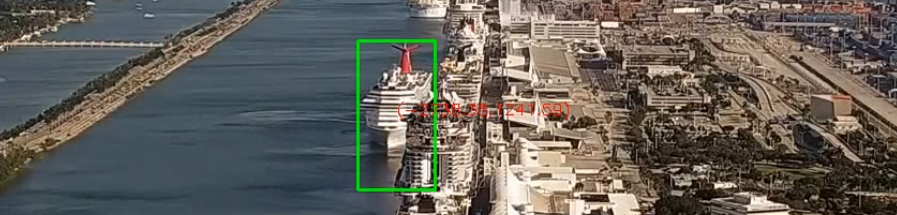
Using the above pipeline inside the video processing loop and drawing each body in bodies will give you something like this:

The simple tracking:

Our simple tracker is just exploitation in the case of no occlusions: we can simply relate the detections from the last frame with the detections from the current frame by just using a threshold of some euclidean distance metric.

# This can be initialized in the class instantiation
trackers = list()
metric_threshold = 0.2

# Here is the processing pipeline
# Map the correspondency between the new bodies and the trackers:
tracker_correspondency = list([None] * len(trackers))
for t in range(len(trackers)):
  for b in range(len(bodies)):
    metric = compute_iou(trackers[t].bbox, bodies[b])
    if metric > metric_threshold:
      if bodies[b] not in tracker_correspondency:
        tracker_correspondency[t] = bodies[b]
        break

# Update all trackers
for t, tracker in enumerate(trackers):
  bbox = tracker_correspondency[t]
  trackers[t][1] = bbox

# Add new detected bodies
for bbox in bodies:
  if bbox not in tracker_correspondency:
      tracker_id = last_id + 1
      tracker = [tracker_id, bbox]
      trackers.append(tracker)
      last_id = tracker_id

The metric used here is the Intersection over Union (see here), but could be also the distance between centroids:

def compute_iou(rect_a, rect_b) -> float:
  """ rect_a and rect_b: [x, y, w, h]
  return: intersection over area (iou)
  reference: http://jsfiddle.net/Lqh3mjr5/ """
  
  xa1, xa2 = rect_a[0], rect_a[0] + rect_a[2]
  ya1, ya2 = rect_a[1], rect_a[1] + rect_a[3]
  xb1, xb2 = rect_b[0], rect_b[0] + rect_b[2]
  yb1, yb2 = rect_b[1], rect_b[1] + rect_b[3]
  area_i = max(0, min(xa2, xb2) - max(xa1, xb1)) * max(0, min(ya2, yb2) - max(ya1, yb1))
  
  area_a = rect_a[2] * rect_a[3]
  area_b = rect_b[2] * rect_b[3]
  
  area_u = area_a + area_b - area_i
  return area_i / area_u

Note that if occlusion occurs, it could, wrongly, swap the targets! But keep calm, it is not the case here :)

Narrowing the detection with masking

Another technique we can apply here is to search for ships only in the port channel, and we can do this by masking with OpenCV’s bitwise operations like bitwise_and:

# Describe each vertice
vertices = np.array([
  [500, 190], # top left
  [575, 190], # top right
  [535, 720], # bottom right
  [0, 720], # bottom left
  [0, 520], # middle left
], np.int32)
vertices = vertices.astype(np.int32).reshape((-1, 1, 2))

# Create a polygon from vertices	 
mask = cv2.cvtColor(frame, cv2.COLOR_BGR2GRAY) * 0
mask = cv2.fillPoly(mask, [vertices], (255, 255, 255))

frame = cv2.bitwise_and(frame, frame, mask=mask)

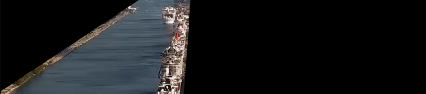
The mask can be seen in the following image:

Conclusion

By applying the described techniques on a simulation where we speed up 60 times the video instead of waiting for the time of the unprocessed frames, we were able to run at around 80 fps on a modern desktop (for instance, it’s an AMD Ryzen 3700x). For comparison, on the same machine, a simplified YOLOv3 was running at around 18 fps.

One can think that if we take into account that we are processing 1 of every 60 frames, wouldn’t we, virtually, be processing a video at 4800 fps? The answer is no, but for live-streaming, we would be freeing the processor for other tasks in the meantime, which is also a great thing!

It is important to point out that despite it being faster than a YOLO, the pipeline used here, applying background subtraction and morphological filters, will probably suffer from a lack of adaptability over different datasets, mostly because, if you notice, it needs some fine-tuning on the parameters to work on specific conditions. This doesn’t mean it is the end for this approach: it is too fast to not be useful. Also, we can architect it in a way that these fine-tuning can be automated using some machine-learning technique or even optimized for a given dataset.